XMF 2: Kinematic Seismic Model Fitter
XMF 2 (Kinematic Seismic Model Fitter) is a platform for "manual" fitting of a two-dimensional layered model to a set of line common shotpoint seismograms. As XTomo-LM, the first application of this product line, XMF is a means of solving the two-dimensional kinematic inverse problem. However, while XTomo-LM implements exact inversion algorithms, XMF is a workframe for empirical try-and-error approach. XMF is released after XTomo-LM, and this is explained by the fact that in some areas, where travel-time analysis is essential, mathematical approach makes excessive demands on input data, while simple well-tested empirical model fitting does work, the more so, that it is built in an appropriate environment. The developers consider both approaches as complementary: both products share the same method of model description and have a program interface, which allows applying them to interpretation of same data. Unlike the first version which offered no technology, XMF 2 contains a large tool kit for approximation of two-dimensional model with a set of one-dimensional sections, fitted each to one seismogram.
XMF input data include a set of common source point seismograms registered on a acquired on a seismic line and, if coordinates of sources and receivers are not written in trace headers, text files with positional information. Seismograms are represented by seismic files of SEG-Y/PC format (that is, SEG-Y adapted to the x86/Windows platform).
Layered model. XMF uses a single two-dimensional curvilinear grid for representation both velocity distribution and seismic boundaries. The grid is stretched on the model wireframe – a set of non-intersecting curves representing seismic horizons. Velocity function is defined at grid nodes, while horizons coincide with some of grid lines. After the user creates or edits the wireframe, XMF stretches velocity grid automatically. The model representation is supported by the relevant ray-tracing algorithms based immediately on the Kirchhoff and Fermat principles.
Components. The following components can be found in the system: basic tools for fitting a model; program framework managing shared data and forcing the user to follow the well-defined iterative procedure; preliminary study (pre-study) – comparatively autonomous unit, implementing the technology of building a 2D model by successive fitting in 1D sections to one seismogram.
Framework organizes user activity as a succession of iterations, each of which includes editing the model, changing wave-layer binding, getting kinematic forward problem solution (i.e. ray-tracing), studying ray picture drawn over the seismograms. The framework represents itself to the user as processing tree whose nodes are XMF projects and iterations. The processing tree is the main GUI device through which the user does his or her work.
Basic tools are programs (modules) running within the framework and solving substantial interpretation problems:
Line seismogram viewer (LSV) allows viewing multiple seismograms, scrolling their views along the line with the arrow buttons, as on fig. 1. The user can adjust trace display and amplitude control and perform reducing seismic record with given reduction velocity. The same module displays computed TX-curves over seismograms allowing the user to estimate how the model fits in the wave field.
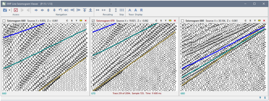 Fig. 1. Seismograms with TX-curves in LSV window.
Graphic model editor consists of two components: geometry editor and velocity editor. The former allows editing the model wireframe, i.e. change shape and position of model horizons. The latter provides for editing velocity graphically and by changing velocity profiles in numeric form. Both editors are equipped with tools for very effective work.
Forward Problem Solver traces rays of diving, reflected and head waves. FPS traces ray for a user-defined samples of waves and sources concurrently to boost productivity. The result is in the Ray Catalog database optimized for fast access to individual rays and ray paths.
Ray Picture Viewer (RPV) provides viewing ray picture by ray samples, which the user composes using criterion composed of conditions on waves, shotpoints, receivers, offsets or model area. The important feature is a tool for examination of ray samples matching TX-curve points on a specified rectangular of a seismogram as shown on fig. 2. On the snapshot, the LSV and RPV windows are displayed. A rectangle on seismogram is selected with the rubber-band; the selected menu command launch RPV, which displays the rays matching exactly the TX-curve points within the rubber-band. The feature helps to bind a TX-curve segment that deviates from a phase line-up to a segment of a seismic boundary or (for the diving wave) to a segment of velocity vertical profile and, in this way, helps the user to correct the model properly.
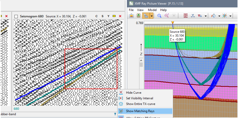
Fig. 2. Ray sample matching TX-curve pints within the rubber-band on the seismic record.
Pre-study provides the technology of fitting, based on constructing 2D model from a set of one-dimensional sections, each of which is built by fitting one of standard models to the wave field of one seismogram. The standard models are associated with the types of waves that can be traced on the seismogram. D-model is associated with the diving wave and used to fit velocity function V(z) for the low velocity zone. R-model is used for fitting a flat reflector; the model parameters are vertical depth, slope and velocity in the overburden. H-модель is associated with head wave and has an additional parameter: boundary velocity value. All models use one-dimensional velocity distribution V = V(z).
Due to simplified assumptions of standard models, getting forward problem solution is instantaneous, while well-designed user interface allows trying a great amount of variants within short time. Standard models are applied within the process of layer-by-layer interpretation resulting in 1D section, which is attached to the vertical passing through the shotpoint of the seismogram. After building the first 1D section, it is used as initial iteration for the next seismogram, reducing fitting time drastically, and so on. This way, a set of 1D sections is built for a sample of line seismograms. In parallel with building 1D sections, a special program constructs from them a 2D model; it can be implanted in the processing tree and so made available for solving two-dimensional forward problem; its solution can be compared with to one-dimensional solutions. In this way, XMF compensates for "loss of dimension".
Pre-study is, naturally, applied to refine the initial model in the zero iteration (that explains the term "preliminary study"). However, pre-study is allowed to start with a model from any project iteration.
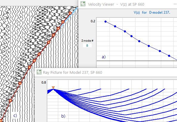
Fig. 3. Pre-study graphic tools : а) velocity profile editor; b) ray picture viewer; c) fitting visualizer.